I recently started to learn Machine Learning from Professor Andrew Ng's Course on Coursera on Supervised machine learning and finished the first week. In this article I will be covering everything I learnt about Linear Regression, Cost Function and Gradient Descent. This blog will cover the topics on a basic level for beginners (like me). I will try to cover more practical examples with code and examples in future.

Prerequisites:

• Basic Understanding of Coordinate geometry, equation of lines

• Some Familiarity with Calculus, Partial derivatives in particular (Optional)

Linear Regression:

Linear Regression is one of the most basic Supervised Learning algorithms. It is a supervised learning algorithm as it makes predictions based on the given data.

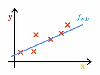
I will be using the example that was used in the course to explain this Algorithm, prediction of house prices with respect to the area of the house in square feet. The image below shows us the data set plotted on the graph, where the price is plotted on the y-axis and the area is square feet is plotted on the x-axis.

Our goal is to make a prediction of the house price where we are given the area in square feet. The best way to do this is to find a best-fit line that is closest to the maximum points in the dataset. This is where Linear Regression helps us. Linear Regression is basically, fitting a line through a dataset that has the least error.

The Math behind Linear Regression:

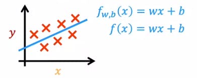
If you are already familiar with Equation of lines, this will be very simple to understand. Recall that the equation of a straight line is y=mx+c. Where m is the slope and c is the y-intercept. We use the same equation as a function to plot the line through our data:

$$f_{w,b}(x)=wx+b$$

In this equation, function f(x) uses x as an input variable and w,b are other function parameters, w is the slope of the line and b is the y-intercept. We or rather, the algorithm adjusts the parameters w and b to find the best fit line.

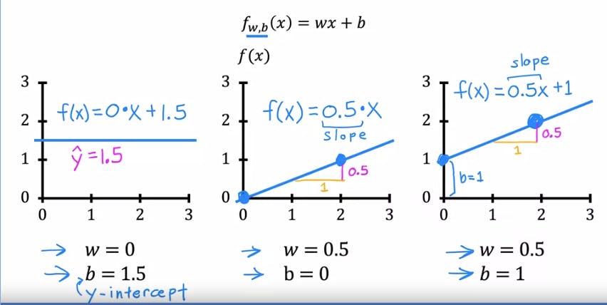
The above image shows the plot for different values of w and b.

This is our sample dataset and we can observe that it is closest to example from the image above, where w=0.5 and b=1. Now you must be wondering how do we find the optimal values of w and b. For this task we create and use something called a cost function.

Cost Function:

We know that:

$$\hat{y}^{(i)}=f_{w,b}(x^{(i)})=wx^{(i)}+b$$

which means that for value of every single value of x there will be a value on y axis, which is the variable y-hat. The cost function helps us choose value of w and b such that the linear regression line passes through almost all points and as is not that far off from the data set points.

Squared error cost function:

$$J_{w,b}={(\sum_{i=1}^m(\hat{y}^{(i)}-{y}^{(i)})^2}/2m$$

The above equation is called the Squared error cost function. Each value of X will corresponds to a value Y-hat on the line. However, our training dataset may also have a corresponding value Y to the same value of X. The difference between these 2 value (y-hat and y) is the error. The goal of linear regression is to find such a line where the value of the error is minimum. Since there are multiple such errors, we need to calculate the mean of this error, and that is what the squared error cost function does. When we minimize the value of the function J, we find the optimal values of w and b.

Visualising the cost function:

Let us fix the value of b as 0 in the equation of the line for our Linear Regression Model. The image below shows us the graph plotted for the values of J(w) which is the cost function when b is constant and we change the values of w, the slope.

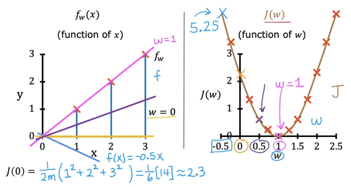
The pink line passes through all the points and therefore is the bestfit line and J(w) is 0 for w=1 for this particular dataset.

If the values of b are not kept constant, and are changed as well, we get a 3 dimensional graph like the one shown below:

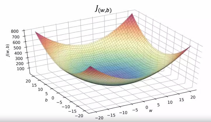
The y-axis represents the Cost function and the horizontal plane axes x and z represent values of b and w. A better way to visualise 3d graphs would be using contours plots.

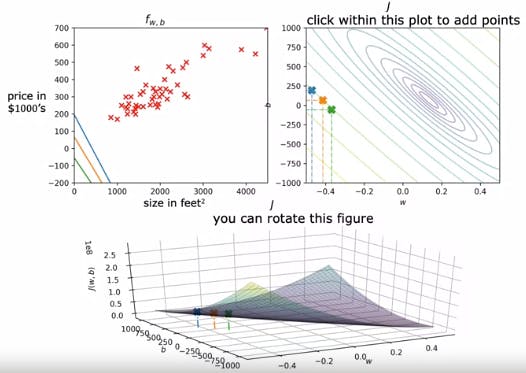
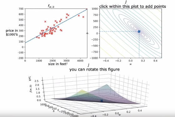
In this figues you can see the given 3d graph is plotted as a contour and the different colours of lines indicate the values of b and w. The value at the centre of the smallest oval shape in the contour plot is the optimal value as it is the lowest value of the Squared error cost function as shown below. This also gives us the best fit line.

Gradient Descent:

Gradient Descent is an algorithm that is used to minimize the any function in a systematic way. Here we will see how it is used to minimize the cost funtion J(w, b) that we saw above. In case the function J, which we are trying to minimize is not a Squared error cost function it may have multiple local minima values and not a single global minima.

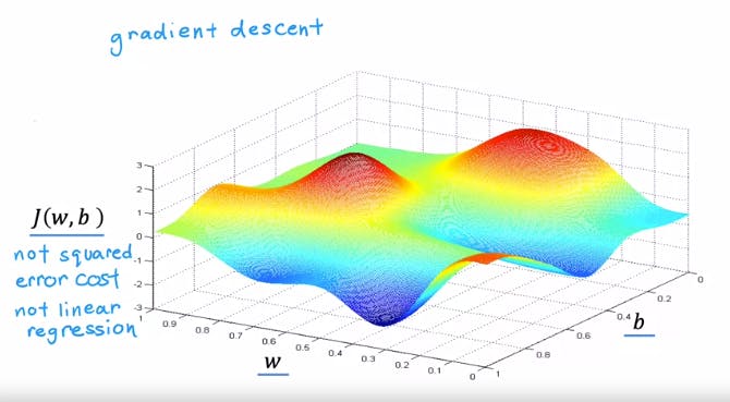
For example, this function has two local minimas or troughs. A function like this can be minimised by gradient descent

The math behind Gradient Descent:

The mathematical equations for the Gradient Descent Algorithm are:

$$w=w-\alpha\frac{\partial }{\partial w}J_(w, b)$$

$$b=b-\alpha\frac{\partial }{\partial b}J_(w, b)$$

Here we are minimising both, the values of w and b. In both the equations, Alpha is the learning rate. You can imagine alpha as the size of the steps we would take down a crest to find a local minima. The value of alpha is usually a small positive value. If the value of Alpha is too high, it may not give us the correct value of the minima and if it is too small, the algorithm would be very slow as the steps would be too small. The partial derivate terms in both equations is the determines the direction and size in which the steps are taken down the graph to find the local minima.

Note that the values of w and b are to be update simulatneously otherwise the algorithm will not work.

$$temp_w=w-\alpha\frac{\partial }{\partial w}J_(w, b)$$

$$temp_b=b-\alpha\frac{\partial }{\partial b}J_(w, b)$$

$$w= temp_w$$

$$b=temp_b$$

As the gradient descent algorithm minimizes a function, the slope of the graph becomes smaller, therefore the partial derivative term will become smaller and as a result of which smaller steps will be taken near the local minima.

Gradient Descent for Linear Regression:

The mathematical formula for Linear regression is a result of partially differetiating the squared error cost function with respect to w and then b.

$$w=w-\alpha{(\sum_{i=1}^m(f_{w,b}(x^{(i)})-{y}^{(i)})x^{(i)}}/m$$

$$b=b-\alpha{(\sum_{i=1}^m(f_{w,b}(x^{(i)})-{y}^{(i)})}/m$$

Remember that practically, the values of w and b are updated simultaneously.

The image above shows us the application of Gradient Descent for different values till it reaches the minima and the Yellow line, which is the best fit line, is achieved.

Since the gradient descent algorithm uses the Cost Function that is based off of the entire training data set, it is called the "Batch" Gradient Descent. There are other Gradient Descent Algorithms that work off of only a subset of the given dataset, however, Linear Regression uses the Batch Gradient Descent.

All the images used are part of the Machine Learning Specialization on Coursera offered by Stanford Univeristy and taught by professor Andrew Ng.